
Charts, tables & diagrams
Data and structure as first-class objects that update with your document — not screenshots dropped onto a slide.
Charts#
Insert a chart (W) and pick a kind from the tool's menu: bar, line, scatter, area, or step. Use Data from in the inspector to choose a table, a function, or an equation. Equation plots support Line and Scatter; follow Plot an equation to vary one input over a range. A figure generated by a code cell is an artifact instead, and redraws whenever the cell reruns.
The inspector controls axes, series, and appearance. PDF and image exports use browser captures at the selected resolution; supported charts can export as native PowerPoint charts, with equation plots retaining numeric x coordinates. Exported charts do not retain their live Quodra connections. See Import & export.
Reading a table#
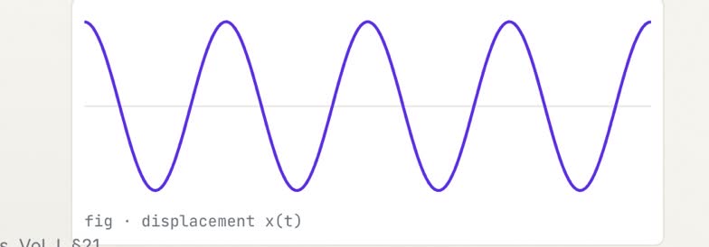
The Data source select lists every table in the deck, or — none —. Reading it is deliberately simple: skip the header row if there is one, take the second column as y and the first as x, and fall back to the row's position when the first column is not a number. So a two-column table of x and f(x) plots as you would expect, and a one-column table plots against its own index.
Until a table chart has a source it says so on the slide — "bind a table — Data source" — rather than drawing invented numbers. In table and function modes, a log Y scale holds zero or negative samples at the smallest positive value in the series. Equation plots require a linear Y axis and report invalid samples instead.
What the inspector controls#
| Section | Controls |
|---|---|
| Type | Bar · Line · Area · Step · Scatter for table or function data; Line · Scatter for an equation. |
| Labels | title, x, y, cap (a caption under the plot), Value labels, Legend. |
| Axes | Fixed min and max — leave them empty and the axis fits the data — plus Y scale Linear or Log, Gridlines, and how many Ticks to draw. |
| Series | Colour, and then whichever applies: Stroke width and Points for the line-like kinds, Bar width for bars, Fill opacity for an area. |
The axis window is bindable: point a parameter at axis minimum or axis maximum and you can open the scale up live. For a table source, drive the table's cells to change the data itself.
For an equation source, axis labels come from its input, output and units. Vary, From, To and Apply range control the sampled interval; other equation inputs retain their current local or linked values. The chart's Legend switch shows its series label. To explain individual symbols, add a separate variable legend.
Tables#
Insert a table (⌘B) for structured values. Edit cells directly; adjust rows, columns, and styling in the inspector.
Click into any cell and type — the grid commits what you leave behind. Rows and Columns resize the grid from the inspector, up to twelve rows and six columns.
- Header row promotes the first row, Row striping bands the rest, and Borders draws None, All or Outer.
- Cell align sets the default, Per column overrides it (Auto, L, C, R), and Numbers right right-aligns any column whose values all read as numbers so they line up on the decimal point.
- Density switches Roomy to Compact, First column sets it Plain or Bold, Text size and Caption finish it.
A table is also the tidiest way to drive a figure without code. Every cell that already holds a number is offered as a binding slot, so a slider can move one value, the chart reading that table redraws, and the decimals the author wrote are preserved — a column reading 1.00, 4.00, 9.00 does not turn into 4.7000000001 the moment it is driven.
A variable legend is a table linked to an equation. Its generated rows, header and values cannot be edited or driven as ordinary table cells. Edit the source equation's definitions instead; table styling remains available.
Diagrams#
The diagram object (in the chart tool's menu) is for structure rather than data — boxes, links, and flows that you arrange on the slide.
Set the number of Nodes (one to twelve) and a Layout: Flow, Tree, Cycle or Force. Flow and tree also take a Direction, Right or Down. Node shape is Round, Box, Pill or Diamond.
Each node has its own label field, wrapped to two lines by the renderer, with Label size and a Highlight that emphasises one node. Edges take their Ends (Line or Arrow), Stroke (Solid or Dashed) and Path (Straight or Curved). Under Appearance: node fill, node edge, edge colour, node size and a caption. The node count is bindable, so a parameter can grow a diagram as you talk through it.
Molecules#
Insert a molecule (from the Insert menu) and give it a structure as SMILES — CN1C=NC2=C1C(=O)N(C(=O)N2C)C for caffeine, c1ccccc1 for benzene. Quodra draws the 2-D structure from the string: bonds, rings, and heteroatom labels are generated, never hand-placed, so the SMILES stays the single source of truth.
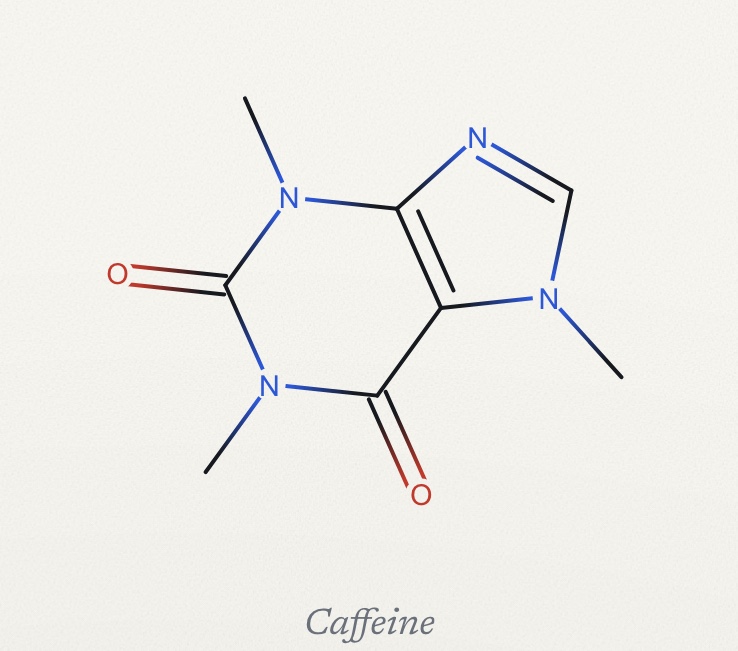
In the inspector you can add a name shown as a caption, colour the heteroatoms (Colour, the conventional CPK scheme) or keep the whole structure in Ink, and draw hydrogens Implicit or Explicit. The generated drawing scales in the editor; PDF, image and PowerPoint exports use image captures rather than retaining an editable molecular structure.
A structure you will use again can go to the library with Save to library. A SMILES the drawer cannot read says so on the slide — "Couldn't read that structure", over "Check the SMILES in the inspector." — and the object stays in place, so fixing the string redraws it.
Drawing in Molecule Studio#
For anything you can’t say in a line of SMILES, open Molecule Studio — press Draw in Molecule Studio in the inspector, or double-click the molecule. It is a full structure editor: pick an element and click to place atoms or change existing ones, drag from an atom to draw a bond, click a bond to cycle its order, and drop a ring template (benzene, cyclohexane, and more) onto empty space or straight onto a bond to fuse it. Add wedge/hash stereo bonds and formal charges, and the formula and SMILES update as you draw. Everything you do rides the deck’s own undo — ⌘Z in the studio steps back your last change — and the structure saves onto the slide when you leave.
Equations#
An equation is an editable object on your slide. Start in Visual to build the expression directly, or choose Linear or LaTeX when you prefer typing source.
Open a screenshot to see the controls at full size. The silent videos cover notation editing, with captions and written steps. For numerical inputs and results, follow Define variables and calculate below.
Create your first equation#
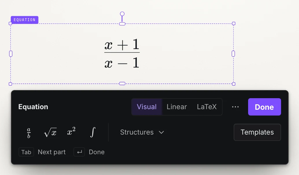
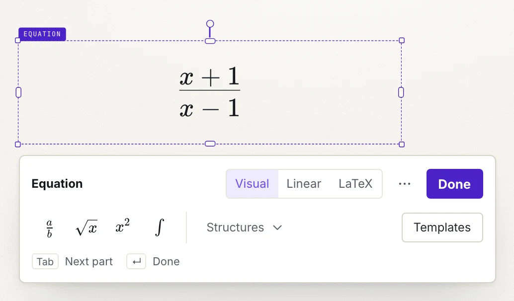
Build a fraction with x+1 above x-1:
- In Deck view, choose Insert → Equation, or press
Ewhile working on the slide. - Keep Visual selected and choose Fraction from the equation toolbar.
- Type
x+1, press Tab to reach the denominator, then typex-1. - Choose Done to finish editing. The fraction stays on the slide as an equation object.
To change it later, double-click the equation, select it and press Enter, or choose Edit equation in the inspector. You can also insert a new equation with ⌘⇧E on macOS or Ctrl+Shift+E on Windows/Linux.
Editing takes place in Deck view. From Canvas, select the equation and choose Edit in Deck; Quodra opens its slide and starts editing there.
Build with structures and symbols#
The toolbar has shortcuts for fractions, roots, powers and definite integrals. Open Structures to find other structures, operators and Greek letters. Select an existing part before choosing a fraction, root or bracket to wrap it.
Typing / in an empty Visual slot opens Structures. After an operand, / remains division input. In the Structures search field, use ↑ / ↓ to choose a result and Enter to insert it.
To create a 3 × 3 identity matrix:
- Start a new equation in Visual, open Structures, search for
matrix, and choose Matrix. - Set Rows and Columns to
3. Keep Brackets set to Square [ ], then choose Insert matrix. - Fill the first row with
1,0,0, pressing Tab after each cell to move to the next. - Fill the second row with
0,1,0, and the third with0,0,1, continuing with Tab between cells. - Choose Done. The result has ones on its diagonal and zeros elsewhere.
Matrices support up to 12 rows and 12 columns. Click a cell before using + Row, + Column, Delete row or Delete column. In matrix settings, Escape returns to Structures; press it again to close Structures.
Start from a template#
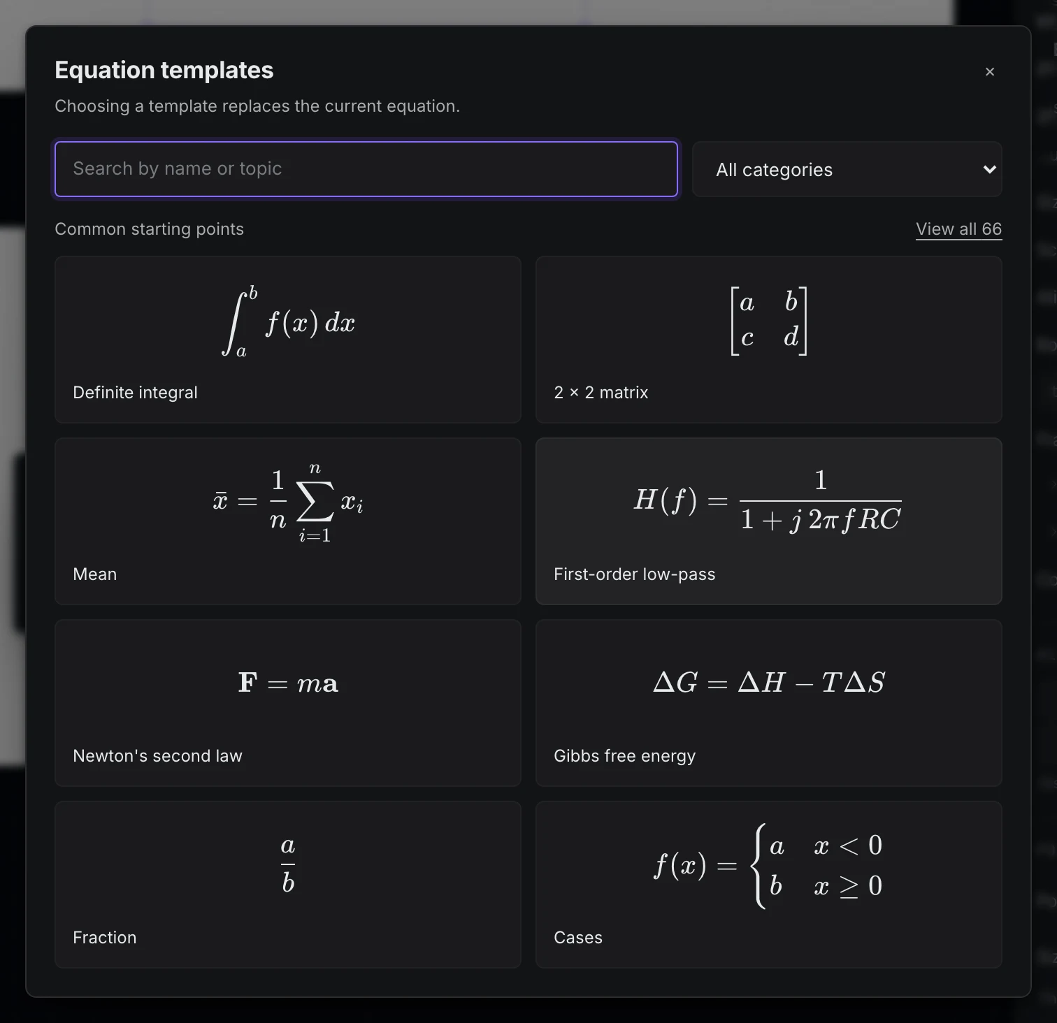
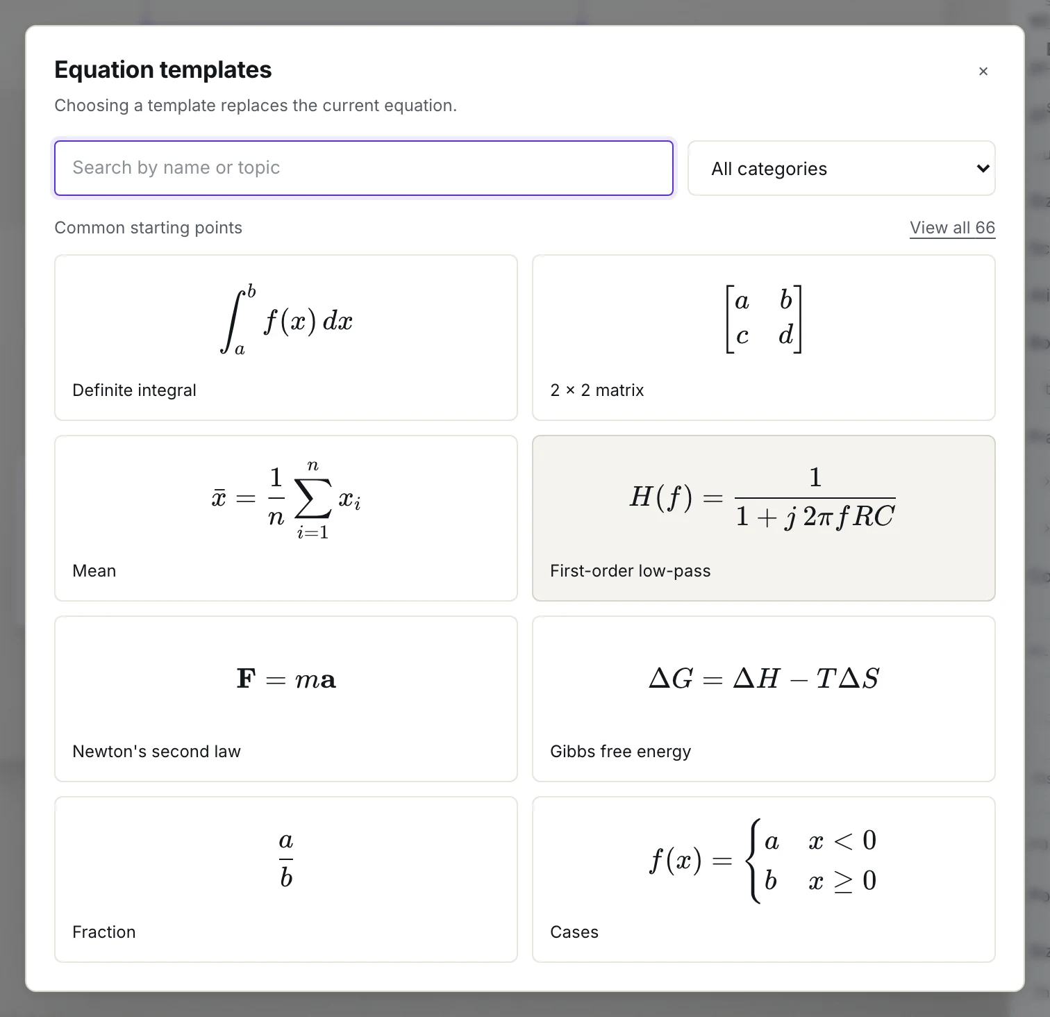
Templates offers complete expressions to adapt. It opens with eight common starting points; use the category filter or View all to browse the rest. Choosing a template replaces the current equation. Undo restores the previous expression.
To use Newton's second law:
- Open an equation and choose Templates.
- Search for
newton. - Choose Newton's second law. The expression
F = mareplaces the current equation and is ready to edit. - Choose Done when you have finished.
For keyboard selection, ↓ in template search focuses the first result; Enter chooses the focused template. Escape closes Templates without changing the equation.
Use Linear or LaTeX notation#
Switch modes in the equation toolbar. Visual edits the typeset expression; Linear accepts compact keyboard notation; LaTeX exposes the mathematical source.
| Expression | Linear input |
|---|---|
| Pythagorean relation | x^2+y^2=z^2 |
| Fraction | (x+1)/(x-1) |
| Definite integral | int_0^5 x^2 dx |
| Quadratic formula | x=(-b+-sqrt(b^2-4ac))/(2a) |
| 3 × 3 matrix | bmatrix(1,2,3;4,5,6;7,8,9) |
In Linear matrices, commas separate cells and semicolons separate rows. Use Shift+Enter for a new line in either source mode.
Quodra refuses a mode switch that would lose notation or formatting. Continue in the mode that can preserve the expression. The … button (More equation actions) contains Copy LaTeX, Undo and Redo, plus the math keyboard in Visual mode.
Navigate and recover an unfinished edit#
| While editing | Action |
|---|---|
| Move between Visual parts | Tab / Shift+Tab. At the field boundary, focus can move to the equation controls. |
| Finish an ordinary equation | Enter or Done. |
| Move down within a matrix | Enter moves to the next row, adding one at the end when the row limit allows it. |
| Finish from within a structure | ⌘Enter / Ctrl+Enter, or Done. |
| Close a menu or leave Visual editing | Escape closes the open menu first, or expands the visual selection before leaving the equation. |
| Undo or redo | ⌘Z / Ctrl+Z; add Shift to redo. |
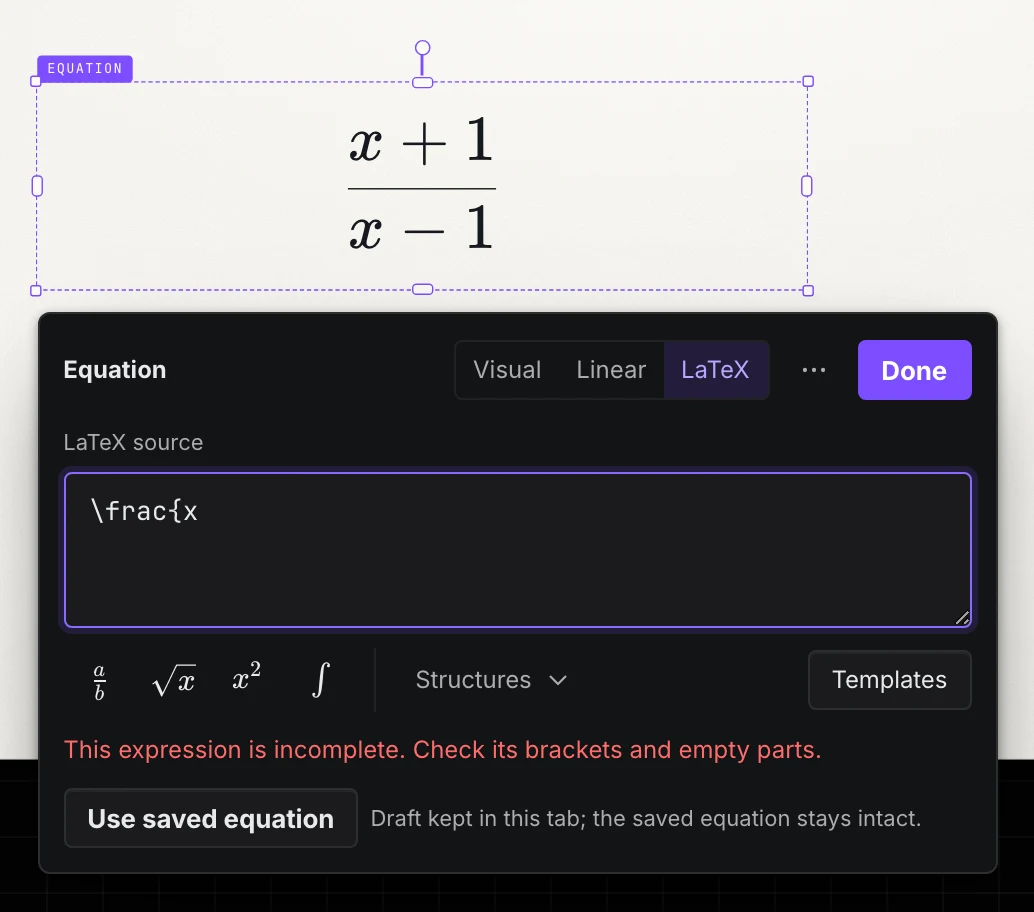
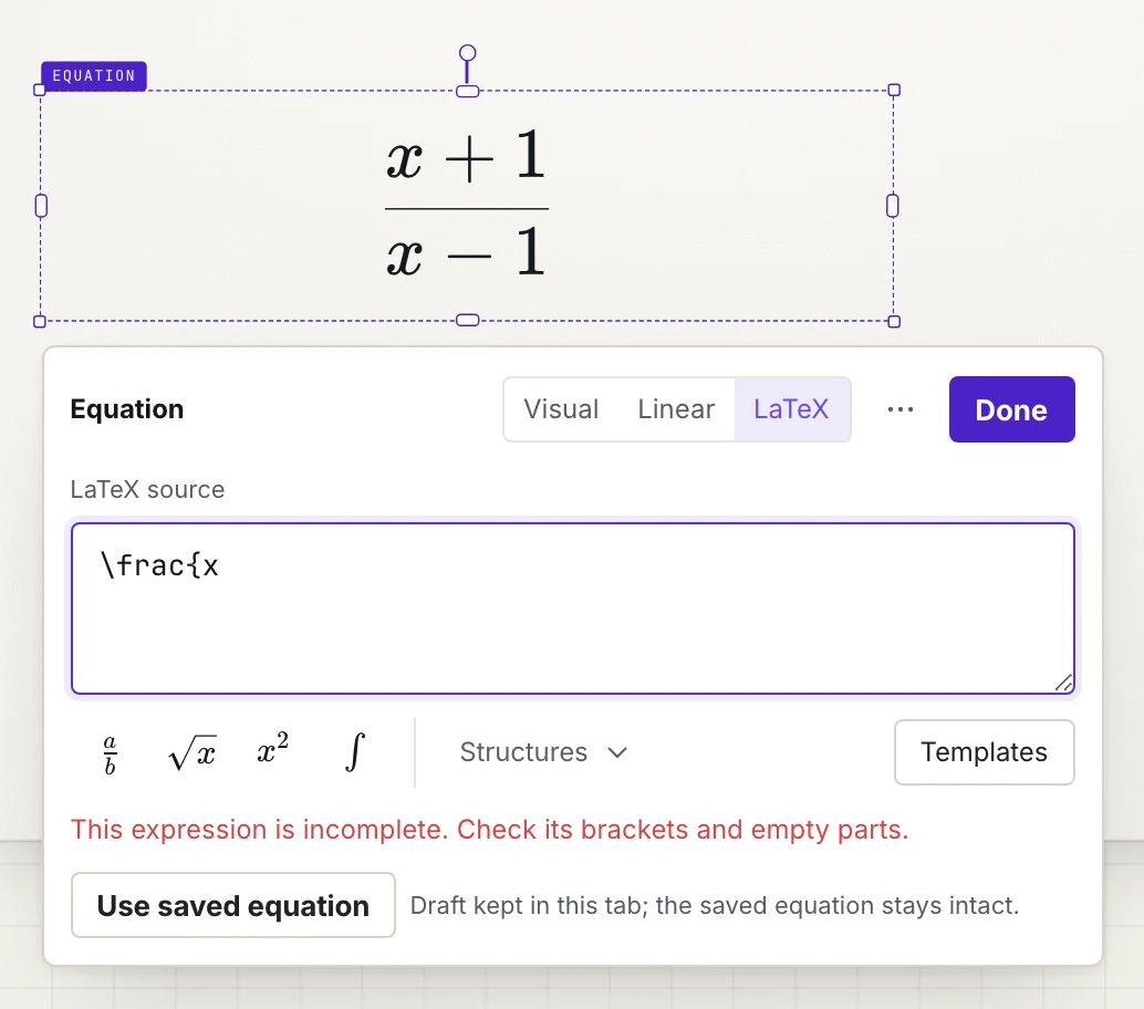
Incomplete or unsupported source keeps the last valid equation visible. Finish the missing part, or choose Use saved equation to discard the unfinished draft. Empty structural slots are allowed in a saved equation; an unknown LaTeX command instead produces a message.
The unfinished draft stays in this tab, including across a reload. It is not a shared or cloud backup. If someone else changed the equation, review the saved version before choosing Apply my draft.
Define variables and calculate#
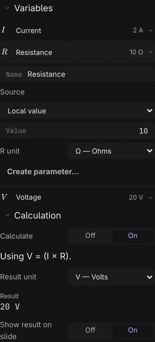
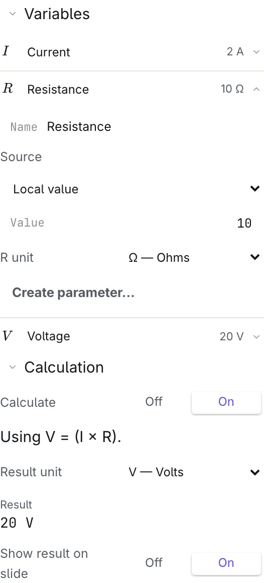
An equation stays symbolic by default. For a supported scalar expression, add local input values and explicitly enable Calculate in the inspector. Calculation produces a numerical result without replacing the authored equation.
Try Ohm's law with current and resistance:
- Create an equation, choose Linear, enter
V=IR, then choose Done. Keep the equation selected. - In the inspector's Variables section, expand
I. Set Name toCurrent, Value to2, and I unit toA. - Expand
R. Set Name toResistance, Value to10, and R unit toΩ. You can name the outputVasVoltage; its value comes from the calculation. - Open Calculation and set Calculate to On. With Result unit → Auto, the result is
20 V. - To display
V = 20 Von the slide, turn Show result on slide on. Turn it off to showV = IRagain. Editing always opens the authored expression.
Input values are saved when you press Enter or leave the field. An empty value is unset, rather than zero. Invalid input shows a message and leaves the saved value unchanged.
The equation's interpretation appears when calculation is on: IR means I × R, with two separate variables. Names such as “Current” explain a symbol; they do not change its notation. Use an explicit multiplication sign when a form could look like a function call, and use a fraction or parentheses to clarify division next to an implicit product.
#### Units and result display
Units come from your input selections, not the letters in the equation. Naming an output V does not establish volts, and m does not imply mass.
For the same example, set I to 2 mA and R to 10 kΩ: the converted result is still 20 V. Choose Result unit → mV to show 20000 mV. Auto derives the result unit; Dimensionless explicitly requires a result with no physical dimension.
The unit menu currently includes:
| Quantity | Supported choices |
|---|---|
| Current, resistance and voltage | A, mA, µA; Ω, kΩ, MΩ; V, mV, kV |
| Mass, length and time | kg, g; m, cm, mm, km; s, ms |
| Area, volume and motion | m², m³; m/s, m/s² |
| Force | N, mN, kN |
| No physical unit | None for an input; Dimensionless for an explicit result choice |
Calculation converts compatible units and checks operations against their dimensions. For example, metres and centimetres can be added; metres and seconds cannot. Products and quotients can produce combined units automatically. These are numerical calculations with finite precision, not exact symbolic results.
#### Let a parameter drive an input
To use a slider instead of a fixed local value:
- Select the equation and expand an input under Variables, such as
IinV = IR. - Open Source and choose an existing numeric parameter. Each option shows its panel, name and current value. Incompatible choices are unavailable.
- With Calculate on, change the parameter value. The equation's result follows it. Show result on slide controls whether the slide shows that result or the symbolic expression.
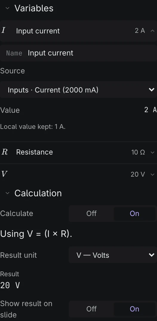
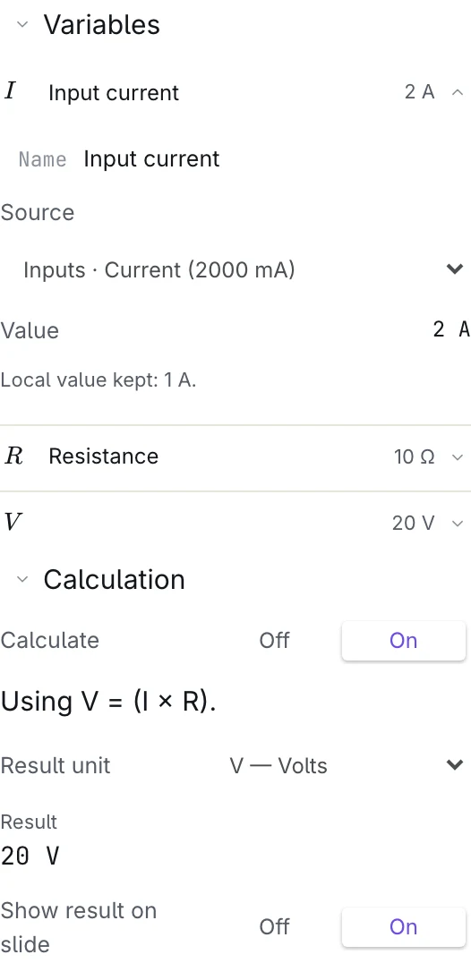
This is a one-way link: the parameter supplies the input, and the equation does not write back to it. Connecting an existing parameter leaves its value, unit and range unchanged. Your saved local value is kept separately; choosing Source → Local value unlinks the input and restores that saved value, not the parameter's latest value.
If the input already has a unit, the parameter must use a compatible unit. Otherwise, the link adopts the parameter's unit. Conversion is automatic: a 100 mA parameter linked to an input measured in A supplies 0.1 A. If the parameter later changes to an incompatible or unsupported unit, the link shows a message instead of reinterpreting the number.
To create a slider from a local input, first set its Value and Unit, then choose Create parameter…. Review Min, Max and Step, and choose Create parameter. The range must contain the current value and the step must be positive. Quodra adds a parameter on the equation's slide and links it in one action; one Undo removes that creation and link.
Renaming or reordering the source parameter keeps the link. Deleting it leaves an unavailable-link message; Quodra does not silently switch to another parameter or fall back to the saved local value. Restore the source with Undo, choose another source, or choose Local value to unlink.
When you copy related parameters, equations, plots and legends together, their copies follow the copied sources. Copying only a dependent object within the same deck keeps its original source. Pasting into another deck without the source leaves a missing link to reconnect there.
#### Plot an equation
Use a plot to show how one input changes an equation's output. For V = IR, vary current while keeping resistance fixed:
- Select the equation and define
Ras10 Ω. Set the inputIunit toA. - In Linked objects, choose Plot equation….
- Set Vary to
I, From to0and To to4. Check that the range unit isA, then choose Create plot. - The new line chart shows voltage from
0 Vto40 V. ChangeRlocally or through its linked parameter to update the curve.
The range replaces the plotted input's value only while sampling. It does not move a linked slider, change the saved local value, or turn Calculate on. All other inputs must have valid current values. The plot uses the same scalar grammar and unit checks as calculation; it does not rearrange equations or evaluate functions that calculation does not support.
Select the chart to change Source equation, Vary, From or To, then choose Apply range. The inspector's Open equation returns to the source. A saved range keeps its unit: compatible input-unit changes convert correctly, while a change of physical dimension requires you to review the endpoints and explicitly confirm the new range unit.
Plots use 81 evenly spaced samples by default, with additional checks between them. A nonfinite or invalid sample, missing source, incompatible unit or detected denominator sign change makes the whole plot unavailable. Quodra does not drop invalid points and draw a line across the resulting gap. Adjust the range to a valid interval. Sampling cannot prove that every point between samples is valid or that a curve is continuous.
Equation plots currently support one input and one output, Line or Scatter, and a linear Y axis. They stay linked to the equation while editing and presenting. In PowerPoint they become static native XY charts with the sampled numeric coordinates.
#### Add a variable legend
Select an equation and choose Linked objects → Add variable legend. A table appears with Symbol, Meaning and Value columns. Meanings use the names you entered under Variables; input values follow their local or linked sources, including units.
The output row shows a result only when Calculate is on. Otherwise it says Not calculated. Missing inputs say Not set; broken links or invalid calculations show Unavailable with a message. Quodra does not infer meanings from letters or evaluate a written meaning as a spreadsheet formula.
Use Open variable legend to select the existing table. Its inspector lets you change Source equation, return with Open equation, and adjust table styling. Generated rows and values follow the source; edit the equation's definitions to change them. In PowerPoint the current legend becomes an ordinary static table.
#### Supported expressions and recovery
Use one isolated output symbol on the left, such as V = IR or I = V/R. The right side supports decimal numbers, single-letter or Greek variables, simple subscripts, arithmetic, fractions, powers and roots. Root indices must be integers from 2 to 12; quantities with units need integer powers or compatible roots.
Calculation does not rearrange an equation to find an unknown. For example, entering V and R into V = IR does not solve for I; write I = V/R first. The output cannot also occur on the right. Functions, integrals, sums and matrices can be displayed but are not evaluated here. Symbolic transformations are not available. Constants such as e or π are not assigned values automatically.
Missing values, incompatible units, division by zero and unsupported notation produce a message. If a result cannot be shown on the slide, Quodra shows the authored equation with the message instead. Neither calculation nor its warnings overwrite the source. Turning Calculate off keeps the definitions for later use.
Definitions belong to this equation object. The same letter in another equation is independent unless you explicitly link both inputs to the same parameter. Links currently accept numeric parameter inputs; other objects, Python outputs and equation outputs cannot supply them.
Changing the expression keeps unused definitions and inactive links under Other definitions. Choose Local value to remove an inactive link, and Remove definition to remove its saved local definition. An unused link does not affect the current result.
Adjust appearance and accessibility#
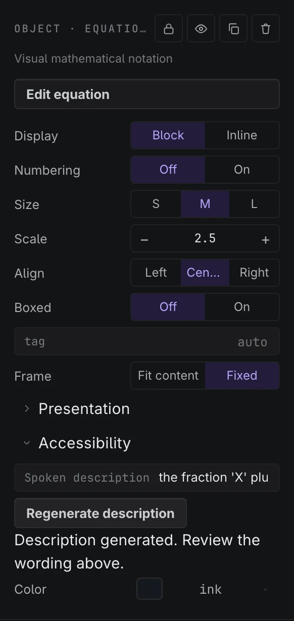
Select the equation to use these inspector controls:
- Display chooses Block or Inline; Size (S, M, L), Scale, Align and Color adjust its presentation.
- Numbering follows the numbered equations on the current slide. A written tag, such as
3.2orA.1, overrides that number. Boxed adds a border around the expression. - Frame → Fit content allows automatic height; Fixed keeps the chosen frame. Corner handles scale the equation proportionally, while side handles adjust the frame.
- Under Accessibility, choose Generate description, then review and edit the spoken description. After changing the equation, Regenerate description replaces the previous description with a fresh reading.
Reveal an equation while presenting#
For a Deck presentation, choose Presentation → Reveal → Fade in the inspector. Slide entry reveals the whole equation when its slide appears; On click reveals it on the next presentation advance. Set the duration in milliseconds.
Static exports and public readers show the complete equation. These controls do not animate individual terms or mathematical transformations.
Display a deck parameter value#
In LaTeX mode, use {{name}} to display a parameter's current value. These references remain in the saved source; Visual and Linear editing are unavailable when they cannot preserve them. A reference displays the value without evaluating the equation. Equations containing these references are not supported by scalar calculation; use an input's Source control when you want a parameter to drive a calculated equation. For computations outside the supported equation grammar, use supported parameter readouts or Python cells.
Citations#
A citation is a reference object rather than a line of hand-typed text. Fill in a citation key, title, authors and year, and then whatever the source has: the journal or book it appeared in, a publisher, volume, pages, a DOI, a URL and a note.
Style switches the rendered line between APA, MLA and IEEE, and the reference is re-formatted for real — the selector is not decoration. IEEE also takes an Index, the bracketed number the line is cited by. A DOI renders as a link to doi.org; a URL is used when there is no DOI.
Images and shapes#
- Image (
M) — bring in a picture when you genuinely need one. - Shape (
R) — rectangle, circle, or line, from the shape tool's menu, for annotation and layout.
Every object also carries the generic appearance controls — fill, corner radius, shadow, opacity — plus a name, and lock and hide switches.
A hidden object is skipped when presenting and on the canvas, which makes it a reasonable place to park the working version of a figure while the finished one is on show. A locked object still renders; it simply refuses to be dragged.
Prefer a native object over an image wherever you can. A chart or equation object stays editable, reactive, and sharp; an imported picture is frozen.
Which one to reach for#
- Numbers you will edit on the slide, or drive from a slider — a table, with a chart reading it.
- A supported scalar equation's response to one input — an equation plot, with a variable legend to explain its symbols.
- Numbers that come out of a calculation — a code cell and its attached figure, or an artifact fed by the cell.
- Relationships rather than magnitudes — a diagram.
- A measured pattern with an instrument's conventions — a Matter Lab object, not a chart. See Matter Lab.
Next#
- Python & code — feed a figure from real computation.
- Circuit Studio — a specialised figure that also solves.